Template : GitHub Link.
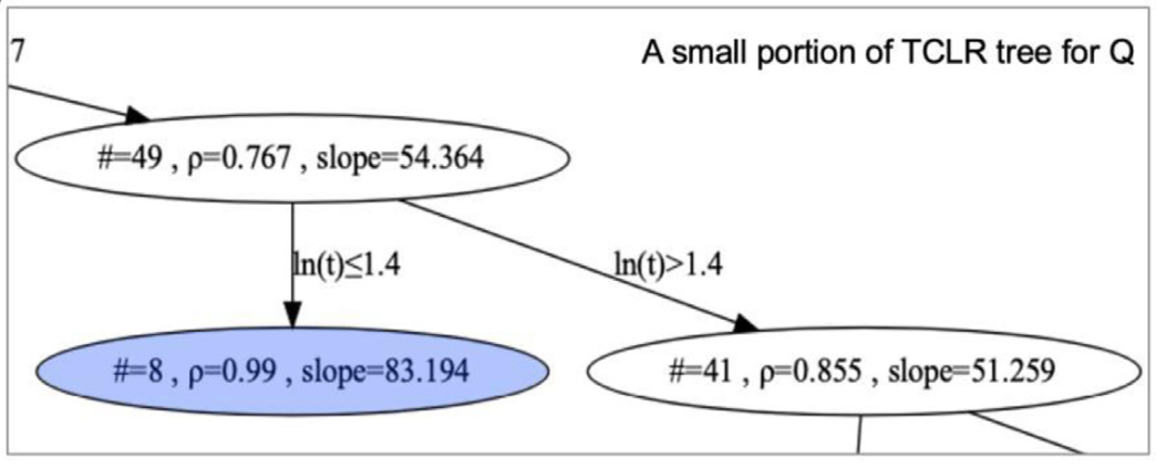
TCLR structure
Please refer to the literature link for the structure of the TCLR model 🔗 TCLR Link.
Intro
In the article titled "Domain knowledge-guided interpretive machine learning: formula discovery for the oxidation behavior of ferritic-martensitic steels in supercritical water" (Paper Link)
Cao et al. introduce an oxidation Arrhenius equation that can be used to predict the oxidation behavior of various ferritic-martensitic steels. This equation can be used to model the oxidation behavior of different alloys and offers insights into the underlying mechanisms of oxidation in these materials.
After omitting the thermodynamic term, a kinetic formula that describes a generalized oxidation thermokinetic equation is derived as formula 1.
formula 1 : ln(W) = n x ln(t) + ln(K)
In which :
W is oxidation weight gain (mg/dm^2) | K is kinetic constant | n is time exponent | t is corrosion time (h)
formula 1 is the logarithmic form of the kinetic equation formula 2
formula 2 : W = K x t ^n
formula 2 is used to describe the oxidation process of a specific alloy: the change of oxidation weight gain over time
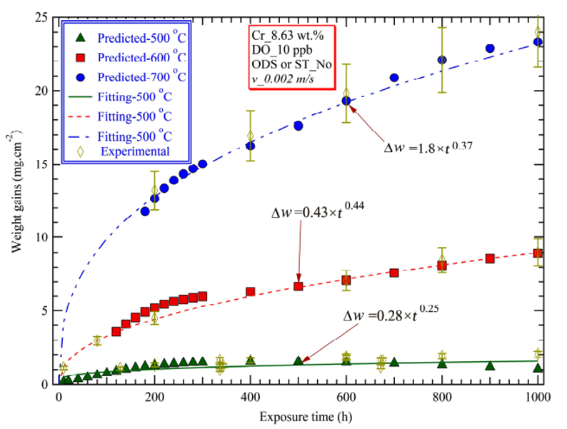 (Figure 1 : Image source)
The time exponent n is affected by alloying elements (Cr, Fe, Mn, ...(wt.%)), test conditions (i.e., temperature T(K) etc.)
The study (Paper Link) conducted by the authors aimed to identify a visual mapping between the time exponent n, alloy composition elements, and test conditions in order to establish a unified expression for describing alloy oxidation/corrosion. The authors sought to derive a formula denoted as f , so that:
formula 3 : n = f(Cr、Fe、Mn、...、T、...)
The identification of the time exponent n, which is a hidden feature in the oxidation dataset, can be challenging. In corrosion tests, it is necessary to obtain a time exponent value by controlling a single variable for a set of alloy oxidation samples. As shown in Table E0:
| Num | fixed | single variable | tests | n |
|---|---|---|---|---|
| 1 | Fe、Mn、...、T、... | Cr = Cr0 | 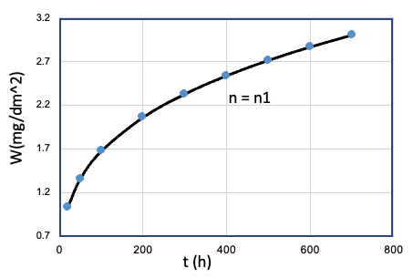 |
n1 |
| 2 | Fe、Mn、...、T、... | Cr = Cr1 | 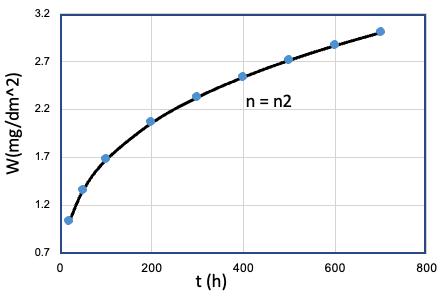 |
n2 |
| ... | ... | ... | ... | ... |
| 10 | Fe、Mn、...、T、... | Cr = Cr10 | 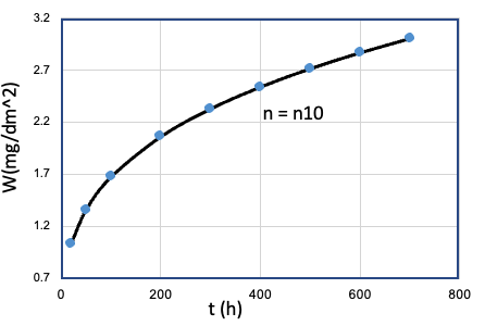 |
n10 |
| 11 | Cr、Mn、...、T、... | Fe = Fe0 | 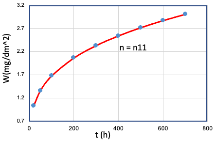 |
n11 |
| 12 | Cr、Mn、...、T、... | Fe = Fe1 | 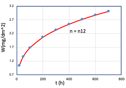 |
n12 |
| ... | ... | ... | ... | ... |
| 20 | Cr、Mn、...、T、... | Fe = Fe10 | 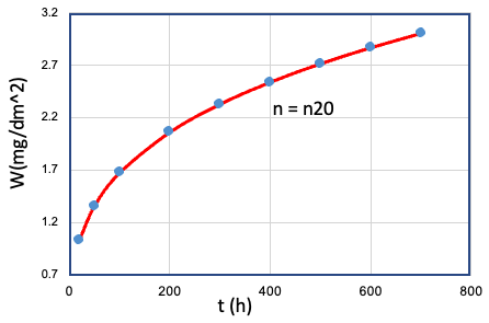 |
n20 |
| ... | ... | ... | ... | ... |
To investigate the relationship between the variablesCr, Fe, Mn,..., T,... and the time exponent n, it is necessary to test each variable individually at different levels while keeping all other variables fixed under a set of given conditions. Each set of data in Table E0 represents the result of a given set of oxidation experiments where a single variable was controlled, and the other variables were kept fixed. However, testing each variable at different levels under different conditions is a challenging and time-consuming task. The large number of combinations required to fully explore the parameter space makes it nearly impossible to provide such a huge experimental sample.
Therefore TCLR was proposed to solve this problem.
The oxidation weight gain of w(mg/dm^2) in Table E1 is a directly measurable variable, and the oxidation dataset shown in Table E1 can be obtained through experimental accumulation (assuming the set size is 200)
| Num | Cr (wt.%) | Fe (wt.%) | Mn (wt.%) | ... | T (K) | t (h) | w(mg/dm^2) |
|---|---|---|---|---|---|---|---|
| 1 | . | . | . | . | . | . | w1 |
| 2 | . | . | . | . | . | . | w2 |
| ... | ... | ... | ... | ... | ... | ... | ... |
| 200 | . | . | . | . | . | . | w200 |
Take the logarithm of the original variable according to formula 1 to get Table E2
| Num | Cr (wt.%) | Fe (wt.%) | Mn (wt.%) | ... | T (K) | ln(t) (h) | ln(w)(mg/dm^2) |
|---|---|---|---|---|---|---|---|
| 1 | . | . | . | . | . | . | ln(w1) |
| 2 | . | . | . | . | . | . | ln(w2) |
| ... | ... | ... | ... | ... | ... | ... | ... |
| 200 | . | . | . | . | . | . | ln(w200) |
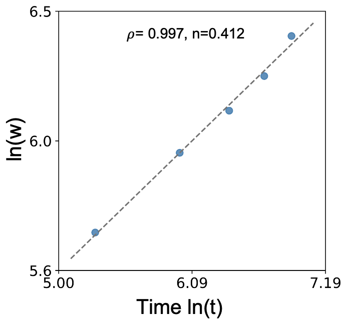
According to the results of formula 1, the slope of ln(W) and ln(t) is the time exponent n
TCLR divides all the data in Table E2 into different subsets according to their characteristics, which is called a leaf. On each leaf, the data conforms to the description of the same time exponent n, that is, satisfies the same dynamic equation.
 (Figure 2 : Image source)
The data points in the figure 2 have different characteristics Cr, Fe, Mn, ..., T, ..., and all satisfy the same kinetic equation exponent n. Therefore, the mapping relationship between the two can be easily obtained. This relationship can be formulated or modeled (described by a surrogate model), resulting in formula 3. Based on this, Cao et al. established a unified equation for describing the oxidation behavior of various alloys under various test conditions.
Template
#coding=utf-8
from TCLR import TCLRalgorithm as model

dataSet = "testdata.csv"
correlation = 'PearsonR(+)'
minsize = 3
threshold = 0.9
split_tol = 0.8

model.start(filePath = dataSet, correlation = correlation, minsize = minsize, threshold = threshold,
            mininc = mininc ,split_tol = split_tol,)
Output:
-
classification structure tree in pdf format (Result of TCLR.pdf)
-
a folder called 'Segmented' for saving the subdataset of each leaf (passed test)
| Result | classification structure | folder |
|---|---|---|
 |
 |
Required parameters for TCLR : dataSet 、 correlation 、minsize 、threshold
dataSet- The studied dataset 「Table E2」.correlation- Association of TCLR features and TCLR variables.minsize- The minimum amount of data on the leaves of the TCLR structure treethreshold- Stop threshold
dataSet :
In order to properly represent the underlying relationships between the features in the incoming dataset Table E2, it is necessary to place the features that contain hidden variables in the last two columns. This approach ensures that the relationships between the features are accurately captured and that the hidden variable is properly accounted for.
For example, in the given problem, the logarithmic time ln(t) and the logarithmic weight gain ln(W) contain a hidden variable represented by the equation ln(W) = n x ln(t) + ln(K). To properly capture this relationship, the variable ln(t) is placed in the penultimate column, while the response variable ln(W) is placed in the final column of Table E2.
correlation :
Define the relationship between variables, in this example, ln(W) vs. ln(t) --> n is linear, and n>0, so define correlation = 'PearsonR(+)' to capture the positive linear relationship .
correlation defined in TCLR: {'PearsonR(+)','PearsonR(-)',''MIC','R2'} :
- 'PearsonR(+)' : to capture the positive linear relationship
- 'PearsonR(-)' : to capture the negative linear relationship
- 'MIC' : to capture non-linear relationship
- 'R2' : to capture non-linear relationship
minsize :
The minsize parameter determines the minimum number of data points required on a straight line in Figure 2, which is obtained by plotting the natural logarithm of the weight ln(W) against the natural logarithm of the time ln(t). To obtain an accurate slope n through the variable ln(W) vs. ln(t), minsize is used to limit the number of data points on the line. The default value of minsize is set to three, meaning that at least three different values of ln(t) are required on a straight line to calculate the slope n accurately.
threshold :
The TCLR uses the threshold parameter to ensure that the data on each leaf is consistent with the same time exponent n.
When threshold is set to 1, all the data on the leaves must fall strictly on a straight line to be considered consistent. In this case, even a slight deviation from the line would be considered inconsistent.
However, in practice, the data is often noisy, and it may be difficult to fit a straight line perfectly. Therefore, the default value of threshold is set to threshold = 0.9. This value allows for some degree of deviation from the straight line while still maintaining consistency in the time index.
Setting the threshold parameter to a value that is too large, such as 0.99 or 0.98, can be problematic. In this case, a large amount of data may not meet the strict condition imposed by the threshold parameter, making it difficult to separate the data reasonably in the TCLR algorithm. This can result in poor performance and inaccurate results.